 1
1 2
2 3
3 4
4 5
5 6
6 7
7 8
8 9
9 10
10 11
11 12
12 13
13 14
14 15
15 16
16 17
17 18
18 19
19 20
20 21
21 22
22 23
23 24
24 25
25 26
26 27
27 28
28 29
29 30
30 31
31 32
32 33
33 34
34 35
35 36
36 37
37 38
38 39
39 40
40 41
41 42
42 43
43 44
44 45
45 46
46 47
47 48
48 49
49 50
50 51
51 52
52 53
53 54
54 55
55 56
56 57
57 58
58 59
59 60
60 61
61 62
62 63
63 64
64 65
65 66
66 67
67 68
68 69
69 70
70 71
71 72
72 73
73 74
74 75
75 76
76 77
77 78
78 79
79 80
80 81
81 82
82 83
83 84
84 85
85 86
86 87
87 88
88 89
89 90
90 91
91 92
92 93
93 94
94 95
95 96
96 97
97 98
98 99
99 100
100 101
101 102
102 103
103 104
104 105
105 106
106 107
107 108
108 109
109 110
110 111
111 112
112 113
113 114
114 115
115 116
116 117
117 118
118 119
119 120
120 121
121 122
122 123
123 124
124 125
125 126
126 127
127 128
128 129
129 130
130 131
131 132
132 133
133 134
134 135
135 136
136 137
137 138
138 139
139 140
140 141
141 142
142 143
143 144
144 145
145 146
146 147
147 148
148 149
149 150
150 151
151 152
152 Effects of cost factor variation
Page 101
Page 102
If you've noticed an error in this article please click here to report it so we can fix it.
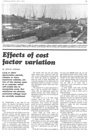
by Johnny Johnson Long or short depreciation periods, cheaper or more expensive vehicles, are two of the choices open to an operator which will enable him to manipulate costs. But whichever he chooses, estimated mileage must be carefully monitored
IN COMPILING a cost table for any vehicle, the operator will discover certain factors which are outside his control and that he cannot influence the cost per week or the cost per mile through manipulating these.
For instance, the cost of fuel is set by the petroleum industry and the Treasury and the fuel consumption of his vehicle by the manufacturer in relation to the engine installed in the vehicle. In effect, therefore, his fuel cost per mile is decided for him.
This is true of most cost factors but such things as depreciation and interest on capital can be varied according to decisions, either to keep his vehicles longer or pay less for them, taken by the operator himself. No wonder, then, that the cost subject which causes more controversy than any other is that of depreciation and the period over which this should be calculated. Is there any merit in quick depreciation and continued operation of the vehicle after the depreciation period has expired or would a long depreciation period make rates more competitive?
The argument for a quick depreciation is that it can be assumed that running a vehicle after the depreciation period has expired provides extra profit because no depreciation charge has to be met during the extended period.
This might be so if all other things remained equal but there is a real connection between depreciation and maintenance costs. During the extended period, the cost of maintenance, which will have been calculated on the same mileage basis presumably as the depreciation, will undoubtedly rise and absorb some if not all of the assumed profit increase.
There might be some merit in depreciating the vehicle over a longer than usual period but the advantage to be gained from this is considered to be marginal.
A simple example might be a vehicle which without tyre price and residual value is depreciated on a capital sum of £3000 over five years and 250,000 mile. This would give a depreciation cost per mile of 1.2p.
If the life of the vehicle were doubled to 10 years and 500,000 miles, the cost per mile would be halved. That is 0.60p a mile. But because the cost of maintenance would increase as the vehicle becomes older and covers a greater mileage some of this saving would disappear. A forecast maintenance cost • per mile of 3p needs only a conservative 10 per cent increase to absorb 0.30p of the saving.
It seems hardly worth while operating vehicles at what would probably be well past their best in order to obtain such a small advantage.
A much better method is to determine the kind of vehicle which suits the particular operation and base the depreciation period realistically. The length of time or mileage which experience has proved to be appropriate to the efficient operation of that vehicle is usually the most economical depreciation period.
This raises the question of whether to buy an expensive vehicle and keep it longer or obtain a relatively cheap vehicle and dispose of it after a short life.
Provided the capital cost is no problem and the only consideration is the difference in operating costs, it is probably more economical to buy the more expensive unit and operate it over a longer period.
To illustrate this it is necessary to realize that if the relative periods of operation were five years for the cheaper vehicle and ten years for the more expensive and one cost only half as much as the other, then there
would be no difference in depreciation costs. But the difference in the cost of vehicles of different design and construction is rarely so conveniently pitched.
Supposing the hypothetical vehicle already used as an example represents the more expensive unit. Over 10 years and 500,000 miles then the depreciation cost per mile would be 0.60p as already demonstrated.
The relatively cheaper vehicle of similar type would probably cost, say £2500 and if it lasted only five years and was operated over 250,000 miles the depreciation cost per mile would be lp and at seven years over 350,000 miles 0.71p.
However, the difference of £500 in original price would reduce the interest to be paid on capital. If this were equivalent to 9 per cent a year, as in CM Tables of Operating Costs, it would result in a reduction of £1 a week in the standing costs or (E1 divided by 1000 miles) 0.10p per mile. The true depreciation cost per mile of the cheaper vehicle at five and seven years would be 0.90p and 0.61p respectively.
In other words, taking the depreciation factor only into account, the possibility is that a further three years' running could be obtained from the more expensive vehicle for the same depreciation cost per mile.
Taking into account the probable trend of maintenance costs, however, the more expensive unit would undoubtedly prove more reliable and cost less in maintenance toward the end of the estimated useful life.
The part played by the estimated mileage which is forecast by the operator as a reasonable assumption of the vehicle's performance is critical. Normally, this estimate will be based on previous years' performances and an intelligent guess about future traffic trends.
The effect of making a forecast that proves to be grossly inaccurate can be serious and it is most important that the mileage being achieved is checked from time to time.
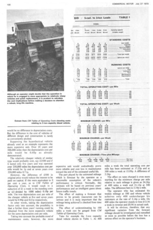
The effect of underestimating by 100 miles a week can be gauged from CM Tables of Operating Costs.
Take for example the 2-ton capacity diesel vehicle shown in Table 1. At 400
miles a week the total operating cost per mile has been estimated at 17.33p and at 500 miles a week at 15.09p. A difference of 2.24p.
The effect on rates charged is even more startling for the minimum charge per mile relative to each mileage is given as 24.26p at 400 miles a week and 21.12p at 500 miles. The difference here is 3.14p a mile.
The operator who has estimated his weekly mileage at 500 and whose vehicle achieves only 400 undercharges his customers at the rate of 3.14p a mile. On 400 miles the operator stands to lose £12.56 a week in revenue and £8.96 in actual cash.
It will be obvious, therefore, that any significant variation from the forecast mileage should be investigated and remedied as soon as possible before the loss has a serious effect on the operator's business.