


COSTS THAT COUNT (8)
Page 43
Page 44
Page 45
If you've noticed an error in this article please click here to report it so we can fix it.
by David Lowe,
MinstTA, AMBIM
IN writing about profits and how they are calculated last week, no mention was made about the special case applying to own-account operators. Many own-account operators, particularly those with very small fleets, pay little attention to costing, are not interested in making a profit from their vehicle operations and, in some cases, are not even unduly concerned if a delivery vehicle is run at a loss.
The latter situation is far from satisfactory and is not, fortunately, too typical. Many of the very large own-account operators have realized the extent to which transport costs eat into total company budgets that they have formed the transport department into a separately accountable division or have even hived the department off as a completely autonomous self-supporting company.
In this case the operation will be carried on almost exactly as a professional haulage business and a profit and specified return on the capital tied up in the operation obtained.
Returning to the usual situation where transport is operated purely as a departmental responsibility within the main company, it is the normal practice for the costs of the transport operation to be looked upon as a "cost of service"; in other words, whatever is necessary to provide the customer either with the service which he requires or to provide him with the level of service promised by the sales force when taking the order is acceptable.
What's needed?
It is still, however, necessary to analyse operating costs to see what the customer service really does cost the company — as opposed to what they assume it costs. It may well be found after suitable investigation that the service being given is better than the customer really needs — in which case a reduction to a more reasonable level will reduce costs — or it may be found that the service costs are out of all proportion to the revenue earned from the customer. In this case a decision has to be taken whether there is any point in continuing to serve that customer. It is purely a question of balancing costs, not against revenue in the way that applies to hauliers, but against the value of the customer's orders.
In calculating the costs of operation, while the profit margin can be omitted from the cost elements, it is important that provision should be included which allows for a return on the capital invested in the transport department as a whole (ie vehicle workshops, offices and equipment) to be recovered.
When the cost figures of operating the department are related to a cost per ton or per mile for the vehicle operations, the
company can then decide by what amount they are prepared to subsidize deliveries if the full costs cannot be recovered in the price of the goods delivered. Obviously, there is a Limit to the amount by which delivery costs can be subsidized and this may be determined by a breakdown of the cost ingredients of the product's retail price. This comprises the cost of production plus return on production capital, cost of sales plus return on capital involved in sales, cost of delivery plus return on transport capital, a margin sufficient to cover all other overheads and finally a margin of profit.
Since the implementation of the 1968 Transport Act in respect of operators' licences some own-account operators have seen opportunities for carrying goods for hire and reward, very often as return loads. Where this has been the policy then costing is essential to determine what rates to charge and a profit has to be added in the normal way.
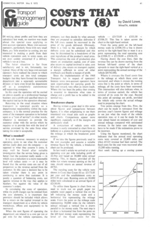
Breakeven charts
Having written a great deal in this series about figures and comparisons between figures, it is often enlightening to see them translated into visual aids such as graphs and charts. Comparisons appear more significant, especially so if the margins are particularly small.
A comparison of vehicle costs with revenue is easily converted to chart form to indicate at a glance the level in earnings and the mileage at which the breakeven point occurs.
If we take the figures previously used in the cost examples and assume a suitable revenue figure for the vehicle, a breakeven chart can be produced.
In last week's article we arrived at a total operating cost per mile including profit of 22.54p and based on 30,000 miles annual running. This, in theory, provided all the miles run where revenue earning at the full rate, should return an annual revenue of £6762.
The standing costs for the vehicle were shown in Costs that Count (6) as £3173.05 per year and the establishment costs as £333.30 per year. Running costs on 30,000 miles were calculated to an annual figure of £2130.00.
To utilize these figures in chart form we need to mark out on graph paper (or suitable ruled paper) a vertical line on the left indicating the money scale and a horizontal line representing the mileage scale. From the point on the mileage scale representing 30,000 miles (ie the vehicle's annual mileage) a vertical line is drawn parallel to the money scale. The next step is to draw a horizontal line from the point on the left-hand money scale representing the level of the fixed costs for the
vehicle — £3173.05 + £333.30 = £3506.35. This line is taken across the chart to the right-hand vertical.
From the same point on the left-hand money scale (ie £3506.35) a line is drawn acrOss to the right-hand line to meet it at a point representing the total operating cost (ie £3506.35 + £2130.00 = £5636.35).
Having drawn the cost lines, then the revenue line can be drawn starting from the bottom left-hand corner of the chart upwards to meet the right-hand vertical at a point representing the annual earnings of the vehicle (E6762.00).
Where it crosses the fixed costs line is the mileage at which these costs are recovered, and where it crosses the running costs line is the point at which, in terms of mileage, all the costs have been recovered. This intersection will also indicate when, in terms of revenue earned, the vehicle has covered all its costs for the year. Beyond this point all earnings are profit, provided the vehicle only covers the actual mileage used in preparing the chart.
Two points emerge from this. First, the chart can be made in retrospect from the previous year's known figures and mileage to see just what the result of the vehicle operation was; or it can be made for the year ahead based on estimates of cost and annual mileage compared with anticipated revenue. In the latter case changes may have to be made if the estimations prove to be incorrect.
Using the figures mentioned, the chart indicates that the annual total operating costs were covered at 22,800 miles and when £5125 revenue had been earned. The fixed costs for the year were recovered after 15,200 miles running.
Next week: Setting up a costing system BRITISH road transport operators are very fuel consumption conscious, yet few operating companies seem to have any idea at all as to the factors which give rise to good or bad consumption figures.
There is a very real tendency for one operator to preen himself because he is getting 8 mpg out of a particular 32-torn-ter whereas another obtains only 6+ mpg from one of his outfits. However, on looking carefully into the operation involved it may well be found that the 8 mpg man ought to be getting nearer 9 and the 6+ mpg man might fairly he expected only to he getting 6 mpg.
A firm which has done a great deal of research work on the concept of fuel consumption is the Swedish Saab-Scania group and the following comments are based upon the results of their research in this area.
Six basic factors
Scania considers that there are six basic factors which cause fuel to be burnt to give fuel consumption performance. First, there is the engine's own consumption. To this must be added consumption from power losses in power transmission (gearbox, rear axle gear, hub reduction, front-axle propulsion and clutch type); consumption for overcoming air resistance; consumption for overcoming rolling resistance; consumption for overcoming differences in altitude; and consumption for acceleration of the vehicle.
With the engine's own consumption it is considered that, to overcome the engine's inner friction and for the operation of auxiliary units as, for example, fan, injection pump and alternator, a certain power is required. The power needed varies according to the design of the engine. A certain increase of the power needed occurs at a higher rpm.
So, to power transmission. Here the vehicle's gear ratio and changing down system has a great influence on fuel consumption. Trucks with toothed transmission gears (which is normally the case) have a power loss of about 0.982 per toothed gear mesh, says Scania. It adds that a power loss of 10 per cent to 12 per cent is usual for a truck with gearbox and rear axle gear. If there are further reduction elements, such as certain types of hub reduction, the power transmission losses increase. The important point concerning the power transmission is the number of revolutions the crankcase rotates per driven kilometre or mile. A high-geared truck has less crankshaft revolutions than a low-geared truck at the same speed.
Change-down bearing
The combination of the engine output and gear reduction has a decisive bearing on fuel consumption. If the engine output is so low that it is necessary to change down fairly frequently, it entails more crankshaft revolutions per driven kilometre or mile.
The third factor is rolling resistance, which varies with the condition of the road. The greater the rolling resistance, the more output required to overcome it. Fuel consumption varies directly proportionally with rolling resistance. The same phenomenon applies to the vehicle's gross weight. The rolling resistance is normally calculated per tonne of vehicle weight and due to this an increase in the vehicle weight (gross weight) creates a directly proportional increase in the fuel consumption. Each extra tonne of payload increases fuel consumption by 0.072 litres per 10km.
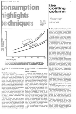
As regards air resistance, Scania rightly points out that the output needed to overcome the air-resistance increases with the square of the velocity. At low velocity the air resistance is insignificant, but as soon as the speed exceeds 50 kmph air resistance begins to influence fuel consumption. The following table shows how the fuel consumption increases at increased speed.
Scania says that, to obtain the total fuel consumption, it has empirically found the following formula: Total consumption = 1.4 + 0.072 X gross weight in tonnes + the speed increase for the desired speed and a given front area.
As regards gradient resistance the output needed to transport a vehicle from one level to a higher level depends upon the level difference. If the terminal point lies at approximately the same level as the starting point, the level differences are compensated during the driving of corresponding downward slopes.
Controlled acceleration The manner in which a driver handles a vehicle makes a lot of difference to fuel consumption. In this respect acceleration of the vehicle is a question of the manner of driving. The main difference between two vehicles which are equally heavy and equally equipped is normally obtained by the difference in driving techniques. Without question, the most economical driving means acceleration in a controlled fashion and deceleration steadily before applying the brakes.
Many drivers, says Scania, accelerate too quickly and are forced to brake heavily. This gives bad fuel economy. The time gain is very little and the wear of the tyres and chassis, in general, increases considerably with stressed driving.
To find out just how bad, and good, driving techniques affect fuel consumption Seania conducted experiments on trial runs in Stockholm over an eight-hour driving period. Each run out and return of the vehicles concerned was 36.3km. A comparison was made on the basis of driving with fuel economy in mind and driving to do the job as fast as possible — in stress conditions in short.
Stress conditions
Under the stress conditions the 36.3km was run in 50 minutes which compared with 52 minutes when driving with fuel economy in mind. With the stress operation, however, a fuel consumption worse by a long way than the economy run was recorded. In one case it was 0.269 litres per km which is roughly 10 mpg and in the other 0.3391cm per litre which is approximately 6.8 mpg. The recorded figurgs on the run showed that the stress driver operated with his foot down for 25km whereas the economy driver operated at full power for 20.7km. Half-power running was reasonably comparable — 6.9krn for the economy driver and 6.61cm for the stressed driver. There was, however, a big difference with foot off the throttle running; in other words the vehicle was rolling. This showed 8km for the economical driver and 2.5 km for the stressed driver. The data also revealed that the latter braked for more than three times the distance of the economy-minded driver; 2.2km compared with 0.71cm.
What better argument for driver training — and refresher courses — than data like this?