


PLANNING A RATES SCHEDULE FOR LOCAL TRAFFIC
Page 24
Page 25
If you've noticed an error in this article please click here to report it so we can fix it.
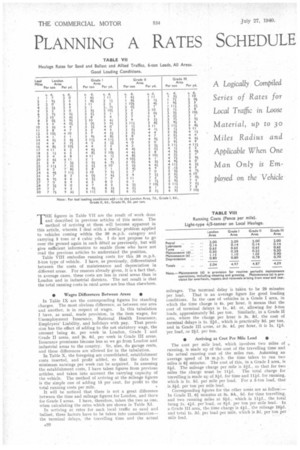
A Logically Compiled Series of Rates for Local Traffic in Loose Material, up to 30 Miles Radius and Applicable When One Man Only is Employed on the Vehicle T" figures in Table VII are the result of work done and described in previous articles of this series. The method of arriving at them will become apparent in this article, wherein I deal with a similar problem applied to vehicles coming within the 30 m.p.h. category and carrying 5 tons or 4 cubic yds. I do not propose to go over the ground again in such claait as previously, but will give sufficient information to enable those who have not read the previous articles to understand the position. Table VIII embodies running costs for this 30 m.p.h. 5-ton type of vehicle. I have, as previously, differentiated between the costs of maintenance and depreciation in different areas. For reasons already given, it is a fact that, in average cases, these costs are less in rural areas than in London and in industrial districts. The net result is that the total running costs in rural areas are less than elsewhere.
• Wages Differences Between Areas •
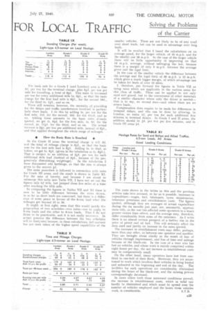
In Table IX are the corresponding figures for standing charges. The most obvious difference, as between one area and another, is in respect of wages. In this tabulation I have, as usual, made provision, in the item wages, for Unemployment Insurance, National Health Insurance, Employers' Liability, and holidays with pay. That provision has the effect of adding to the net statutory wage, the amount being 4s. per week in London, Grade I and Grade II areas, and 3s. 6d. per week in Grade III areas. Insurance premiums become less as we go from London and industrial areas to the country. So, also, do garage rents, and these differences are allowed for iii the tabulation. In Table X, the foregoing are consolidated, establishment costs inserted, and profit added, so that the data for minimum earnings per week can be acquired. In assessing the establishment costs, I have taken figures from previous articles, and taken into account the carrying capacity of the vehicle. The method of arriving at the mileage figures is the simple one of adding 15 per cent, for profit to the total running costs per mile. It will be noticed that there is not a great difference between the time and mileage figures for London, and tho,e for Grade I areas. I have, therefore, taken the two as one, when calculating the rates which are shown in Table XI. In arriving at rates for such local traffic as sand and ballast, three factors have to be taken into considerationthe terminal delays, the travelling time and the actual mileages. The terminal delay is taken to be 20 minutes per load. That is an average figure for good loading conditions. In the case of vehicles in a Grade I area, in which the time charge is 4s. per hour, it means that the cost of terminal delays is Is, 4d. or, allowing for 5-ton loads, approximately 3d. per ton. Similarly, in a Grade II area, where the charge per hour is 3s. 8d. the cost of terminal delays is ls. 21d., which is practically 3d. per ton, and in Grade III areas, at 3s. 4d. per hour, it is 1s. lid. per load, or 2id. per ton. • Arriving at Cost Per Mile Le.ad • The cost per mile lead, which involves two miles of running, is made up of the cost of the travelling time and the actual running cost of the miles run. Asiuming an average speed of 18 m.p.h. the time taken to run two miles is 65 minutes. The cost of this, in a Grade I area, is 50. The mileage charge per mile is 50., so that for two miles the charge must be 11 id. The total charge for travelling is made 'IF of 51c1. for time and 110. for running, which is is. 5d. per mile per load. For a 5-ton load, that is 31d. per ton per mile lead. Corresponding figures for the other areas arc as follow:In Grade II, 61 minutes at 3s. 8ds, 5d. for time travelling. and two running miles at 5id., which is 1Iid., the total being is. 4id. per'load, or aid. per ton per mile lead. In a Grade III area, the time charge is 40., the mileage 10id. and total Is. 3d. per load per mile, which is 3d, per ton per mile lead. The basic rate for a Grade I (and London) area is thus 3d. per ton for the terminal charge, plus Sid. per ton per mile for travelling, a total of 61c1. This must be increased per ton for every additional mile by 34d., so that the basic charge for the first lead mile is 64d., for the second I0d., for the third Is. lid., and so on.
There still remains, however, the necessity of providing for the delays and traffic interferences involved in particularly short leads. I do this by adding Is. per ton for the first mile, lid, for the second, 10d. for the third, and so on. Adding these amounts to the basic rates already quoted, we get Is. 6id, for the first mile, Is. 9d. for the second, is. Hid. for the third, and so on. The actual increase is 2id. per ton per additional mile, instead of Sid,, and that applies throughout the whole range of mileages.
• How the Basic Rate is Reached • In the Grade II areas the terminal charge is still 3d. and the total of mileage charge is 31c1„ so that the basic rate for the first mile lead is 6id. Adding 1s. to that, as before, we get Is. WI. (given in the tabulation as is. 6id.). That is subject to an addition of 21d. per ton for each additional mile lead (instead of 3id., because of the pro
gressively diminishing weightage). In the tabulation I have discounted odd farthings, so that the rate is always given to the nearest id.
The same procedure is followed in connection with rates for Grade III areas, and the result is shown in Table XI. For the sake of brevity, and because I am about to submerge this table into Table VII, I have not set out the figures mile 1:4mile, but jumped them five miles at a time after reaching the fifth mile.
In comparing the figures in Tables VII and XI there is seen to be little difference between the rates shown, in so far as short leads are concerned, but there is a difference of some pence in favour of the 6-ton load when the mileages get beyond 15 to 20.
It might, at first sight, seem that this would justify the preparation of two schedules—two rates—one to apply to 5-ton loads and the other to 6-ton loads. That I do not think to be practicable, and it is not really necessary. In actual practice the difference between the two schedules will be dissicated because, in these calculations, full account has not been taken of the higher speed capabilities of the
smaller vehicles. These are not likely to be of any avail over short leads, but can be used to advantage over long leads.
It will be recalled that I based the calculations on an average speed, fin' the larger vehicle, of 15 m.p.h. and for the smaller one 18 m.p.h. In the case of the larger vehicle there will be little opportunity of improving on that 15 m.p.h. average, .without infringing the law, because there is a margin of only 5 m.p.h. between the average given and the legal limit.
In the case of the smaller vehicle the difference between the average and the legal limit of 30 m.p.h. is 12 m.p.h. which gives a much bigger margin, of which advantage can be taken for leads of over 15 miles.
therefore, put forward the figures in Table VII as being rates which are applicable in the various areas for this class of traffic. These can be applied to not only sand and gravel, but to the conveyance of other materials of a similar character where only the driver is needed— that is to say, no second man—and where there are no return loads.
Compensation does require to be made for differences in terminal delays, and this can be done by allowing, in London, an extra Id. per ton for each additional five minutes in terminal delays. In Grade I and Il areas, the addition should be Id. per ton per five minutes, and in . Grade III areas id.
The costs shown in the tables in this and the previous articles take into account, so far as is possible, increases in expenditure—wages, fuel, lubricants, tyres, maintenance, insurance premiums and establishment costs. The figures quoted, although they are averages of actual expenditure during the six months just past, are, necessarily, approximate only, as the war ha affected some operators to a much greater extent than others, and the average may, therefore, differ considerably from some of the extremes. As I write there is an almost certain prospect of a further rise in the price of petrol and oil fuel. This will seriously affect the data used and justify an increase in the rates quoted.
The increases in establishment costs may differ, perhaps, more than any other, as between one operator and another. They are brought about chiefly as the result of loss of vehicles through impressment, and 1Css of time and mileage because of the black-out. In the case of a man who has lost no vehicles, and whose work is mainly comprised within eight hours per day, the net increase in establishment costs may be comparatively small.
On the other hand, many operators have lost from onethird to one-half of their fleets. Moreover, they are accustomed to work which involves their vehicles in being loaded and unloaded at the beginning and end of the clay., The facilities for such operations are considerably diminished during the hours of the black-out, and the earning potrers correspondingly decreased.
In cases where both those untoward conditions prevail, the increase in establishment costs, which in total can hardly be diminished and which must he spread over the number of vehicles employed and the hours those vehicles work, is considerable. S.T.R.