


It pays to monitor
Page 46
Page 47
If you've noticed an error in this article please click here to report it so we can fix it.
costs weekly by Johnny Johnson
Comparing the weekly performance of vehicles using the vehicle cost sheet can highlight the effect of unusual expenditure. How to do this and how to compile a break-even chart is explained in this article.
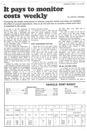
IT is easy to see the importance of knowing how much a haulage job will cost in order that a reasonable and competitive rate might be charged. Equally important, though perhaps not so obvious, is the necessity to see that the costs on which the rate has been based are not exceeded. This involves scrutiny of the weekly cost sheet and intelligent use of the information which it contains to remedy any sizeable variation.
Not only should the performance of the vehicle be considered week by week but also its performance measured against a laid down standard. The standard adopted might be a forecast made by the haulier on the basis of past experience with similar units. For the beginner, the average figures given in Commercial Motor Tables of Operating Costs might be used till a proper dossier of vehicle performance has been built up.
Consider the vehicle cost sheet which is here intended to represent three average weeks in the business of an hypothetical haulier. The figures have been compiled based on CM Tables and they have been deliberately arranged so , as to be unremarkable except for the rather high maintenance expenditure in week ending July 13. Nevertheless, they provide an interesting comparison of the results obtained and the effect of different cost
factors on the week's trading.
It should be borne in mind that the figures are entirely imaginary, however, and the operator achieving a better performance should not take credit nor should the operator whose vehicles do not match the figures shown necessarily be downcast.
Fuel: consumption and cost Taking each of the cost factors shown in order, the fuel consumption achieved is just under 12 mpg, and assuming a residue left in the tank to carry over to the fourth week, will probably exceed this slightly. CM road tests for similar vehicles give an average fuel consumption of 12 mpg so that it can be assumed that the vehicle is functioning well in this department.
So far as fuel cost is concerned, over the period the fuel cost varies from 2.57p a mile to 2.70p a mile which compares well with the 2.63p shown in CM Tables for similar vehicles.
It is difficult to compare the cost of oil in relation to such a short period as that shown but assuming that the gallon bought was toward the end of the week and no more has been bought by the end Of the third week the expenditure shown is reasonable. It is considered the one gallon about every 2000 miles is about average.
Tyre costs are based on the cost of tyres shown in the data given divided by the mileage life of the tyres. This estimated weekly cost has been added in the absence of any actual expenditure.
Maintenance has cost only £15 in the first week against a budgeted cost of £33.60. It is the actual cost which has been added into the total operating cost, the difference being regarded as added profit to the operator.
In the second week, however, the vehicle has incurred a rather heavy maintenance expenditure. The labour cost would probably represent about 18 to 20 hours work which seems somewhat excessive till it is realized that the job was done by two men at weekend and the time shown is really deemed time. That is, each man worked 6 hours on Saturday equivalent to 8 hours at time and a quarter.
Sit up: and take notice
It is figures of this kind that should make the operator sit up and take notice when scanning the vehicle cost sheet. The value of having a number of weeks' figures on one sheet can be appreciated when it is seen how prominently the discrepancy shows up as in the example.
Despite the maintenance cost being so heavy in one week, the overall performance is not disturbing. During the period, the vehicle has achieved a total mileage of 3096 at a total maintenance cost (actual and estimated) of £120 equal to a cost per mile of 3.25p. CM Tables quote an average maintenance cost per mile of 3.36p and the overall result might be considered satisfactory. • As the vehicle is only about 18 months old, however, the prudent operator will make a point of studying the future maintenance figures carefully.
Drivers wages have fluctuated with mileage as would be expected and other standing costs have been added as shown in the summary in the heading of the sheet.
It is interesting to note that the total operating costs per mile have varied slightly each week from just below the standard given in CM Tables •of 14.91p to just above it. Overall, a total operating cost 3f £473.01 divided by a total mileage Df 3096 gives a mileage cost of 15.25p which compares quite well with the standard adopted.
Profit: £50 a week From the weekly trading results, it is deduced that our hypothetical haulier usually enjoys a weekly profit of something of the order of £50. His expenditure on maintenance during the second week has turned this into a loss of £7.39 but the wisdom of having the maintenance jobs done at weekends is reflected in the revenue earned by the vehicle during the week. Had the maintenance been done during the week, it is obvious that the loss would have been considerably greater.
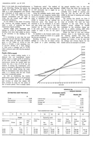
As well as monitoring the weekly performance of the vehicle it is of advantage also to establish the point of mileage and revenue at which the vehicle will have covered its costs for the whole of the 12-month period. This is usually called a "break-even point". The method of determining this point has been described in CM previously but it might be as well to repeat it here.
Using the probable results which might be attained by our imaginary haulier once more, it is possible to show that at 25,000 miles in operation after having earned £5200 in revenue he has reached the break-even point. This should not be assumed to 'be an invitation to sit back and take things easy after it has been reached but it does convey that this is the point after which his business is unable to make a loss on the year's trading.
To establish it, the forecast yearly costs and revenue should be drawn on a graph like the one reproduced.
Standing costs do not increase with mileage so a line can be drawn across the graph at a point coinciding with ' the annual standing cost, in this case £2800. From that point, the running cost can be drawn in. As this haulier will probably incur £4400 in running cost over the year the line will run from £2800 to the total of standing and running cost of £7200.
The revenue line should run from 0 at the base line to the estimated yearly total of £10,400. The total has been calculated, in this case, based on the haulier's annual mileage of 50,000 multiplied by the minimum charge per mile for a vehicle running 1000 miles a week of 20.88p as shown in CM Tables.
Where the lines of cost and revenue intersect, there is the break-even point. By drawing another line from the intersection to either datum line showing mileage and money, it can be seen that the mileage and' revenue figures for the haulier used as an example is as stated.