• Home
• Used vehicles
• Product news
• Dealer news
• Compliance
• Buying advice
• Archive

TESTERS' TWELVEMONTH

by the Technical Editor

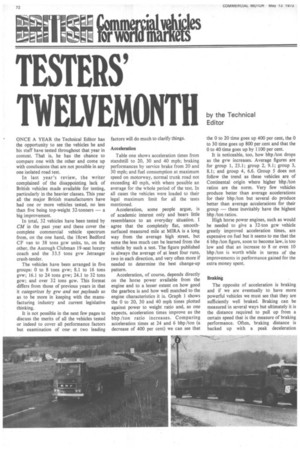
ONCE A YEAR the Technical Editor has the opportunity to see the vehicles he and his staff have tested throughout that year in context. That is, he has the chance to compare one with the other and come up with conclusions that are not possible in any one isolated road test.

In last year's review, the writer complained of the disappointing lack of British vehicles made available for testing, particularly in the heavier classes. This year all the major British manufacturers have had one or more vehicles tested, no less than five being top-weight 32-tonners — a big improvement.

In total, 32 vehicles have been tested by CM in the past year and these cover the complete commercial vehicle spectrum from, on the one hand, the 18cwt Bedford CF van to 38 tons gcw units, to, on the other, the Ascough Clubman 19-seat luxury coach and the 33.5 tons gvw Jetranger crash-tender.

The vehicles have been arranged in five groups: 0 to 8 tons gvw; 8.1 to 16 tons gvw; 16.1 to 24 tons gvw; 24.1 to 32 tons gcw; and over 32 tons gcw. This format differs from those of previous years in that it categorizes by gvw and not payloads so as to be more in keeping with the manufacturing industry and current legislative thinking.

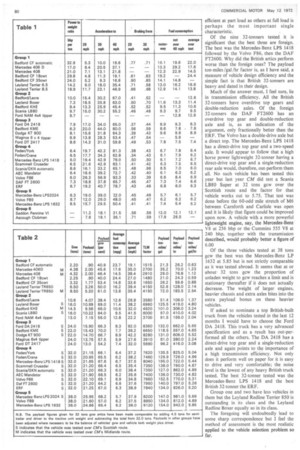
It is not possible in the next few pages to discuss the merits of all the vehicles tested or indeed to cover all performance factors but examination of one or two leading factors will do much to clarify things. Acceleration Table one shows acceleration times from standstill to 20, 30 and 40 mph; braking performances by service brake from 20 and 30 mph; and fuel consumption at maximum speed on motorway, normal trunk road not exceeding 40 mph, with where possible an average for the whole period of the test. In all cases the vehicles were loaded to their legal maximum limit for all the tests mentioned.

Acceleration, some people argue, is of academic interest only and bears little resemblance to an everyday situation. I agree that the completely flat, smoothsurfaced measured mile at MIRA is a long way from the average high street, but none the less much can be learned from the vehicle by such a test. The figure published is always the average of at least four runs, two in each direction, and very often more if needed to determine the best change-up pattern.

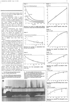
Acceleration, of course, depends directly on the horse power available from the engine and to a lesser extent on how good the gearbox is and how well matched to the engine characteristics it is. Graph 1 shows the 0 to 20, 30 and 40 mph times plotted against power to weight ratio and, as one expects, acceleration times improve as the bhp /ton ratio increases. Comparing acceleration times at 24 and 6 bhp /ton (a decrease of 400 per cent) we can see that the 0 to 20 time goes up 400 per cent, the 0 to 30 time goes up 800 per cent and that the 0 to 40 time goes up by 1100 per cent.

It is noticeable, too, how bhp/ton drops as the gvw increases. Average figures are for group 1, 23.1; group 2, 9.1; group 3, 8.1; and group 4, 6.6. Group 5 does not follow the trend as these vehicles are of Continental origin where higher bhp /ton ratios are the norm. Very few vehicles produce better than average accelerations for their bhp /ton but several do produce better than average accelerations for their group — these inevitably have the highest bhp /ton ratios.

High horse power engines, such as would be needed to give a 32-ton gcw vehicle greatly improved acceleration times, are expensive on fuel but it seems to me that the 6 bhp/ton figure, soon to become law, is too low and that an increase to 8 or even 10 bhp /ton is worth while in terms of the improvements in performance gained for the extra money spent.

Braking The opposite of acceleration is braking and if we are eventually to have more powerful vehicles we must see that they are sufficiently well braked. Braking can be measured in several ways but ultimately it is the distance required to pull up from a certain speed that is the measure of braking performance. Often, braking distance is backed up with a peak deceleration achieved by the vehicle during braking which is by the very nature of things higher than the average deceleration.

Average deceleration, which is easily worked out once the overall stopping distance is known, is useful because it can be used to compare braking performance at any speed. Graph 2 shows average deceleration from 30 mph for the vehicles tested in the past year. It is clear that braking performance deteriorates as vehicle gvw increases.

Individual performances vary considerably owing to road conditions, vehicle types, etc, but the trend is well marked, a 2 tons gvw vehicle can manage 0.7 g whereas a 32 tons gcw vehicle can only manage 0.4 g. At 30 mph 0.7 g is equivalent to a stopping distance of 35ft and 0.4 g to 73ft, ie slightly more than twice the distance.

For comparison a one-ton family car can achieve an average deceleration of 0.9 g — a stopping distance of just over 31ft. To achieve better braking, particularly in the case of a 32 tons gem, vehicle, is technically difficult because of the sheer lack of space to place conventional brakes. A big improvement could only be made by changing to, say, disc brakes or by using an auxiliary braking system. 0.5 g (60ft at 30 mph) can be considered a desirable minimum performance and it is interesting to note that at 32 tons gcw only the Mercedes-Benz LPS 1418 achieves this figure. The Scania automatic, however, achieved 0.46 at 30 mph and 0.69 at 40 mph with the aid of the retarder built in to its GKN automatic gearbox. Vehicles from 22 tons gvw down nearly all bettered 0.5 g.

It is significant that all the Continental vehicles tested were fitted with exhaust brakes. This type of brake, which is not expensive (they are standard equipment on most Continentals), is very useful and often the exhaust brake alone is enough to check the vehicle speed thus saving wear and tear on the service brakes. With the notable exception of Ford no British vehicle tested had an exhaust brake.

Motorways have tended to lift vehicle operating speeds and yet braking performance in Britain at least does not seem to have kept pace. If the brakes themselves cannot be made to perform better the addition of a low-cost exhaust

brake would it seems to me be a good remedial measure. Paradoxically, the vehicles returning the best braking performance with the service brakes were among these with exhaust brakes fitted.

Fuel consumption

Fuel consumption is probably the one performance area producing the most interest among vehicle operators. Traditionally, this is the factor that operators say determines whether they make a profit or a loss. This is obviously not so, for as can be seen from the CM Tables of Operating Cost, fuel only constitutes between 15 and 20 per cent of total operating costs.

The high figure would be typical of a 32 tons gcw artic operating 1000 miles a week, for example. The graph of fuel consumption against vehicle gvw, again of vehicles tested this year, shows that fuel consumption is remarkably consistent within any weight bracket, The variation, for example at 22 tons gvw, is 1 mpg in 8 (12+ per cent), and at 32 tons gcw 0.9 mpg in 6,0 (15 per cent). In other words, variation in fuel consumption is likely to affect overall costs no more than 15 per cent of 20 per cent (3 per cent).

For the great majority of operators using smaller vehicles and doing less mileage the possible variation will be less, some as little as one per cent. The graph of fuel consumption against vehicle gvw shows clearly that the heavier vehicle uses proportionately less fuel — for example, 15 mpg is normal for 8 tons gvw, but the 16 tons gvw vehicle returns 10,5 mpg not 7.5 as might be expected, and the 32 tons vehicle returns 6.4 and not 3.75 mpg as might be expected. This is due mainly to the decreased bhp /ton of the heavier vehicles.

What is important in determining costs is how much payload the vehicle carries, for this directly affects the productivity of the driver's time and of the capital tied up in the truck.

Broadly speaking, truck and driver moving 20 tons is twice as productive as a driver and truck moving 10 tons and 20 times more productive than a driver and truck moving one ton. Admittedly, a 32 tons gcw artic outfit costs more than a one-ton van but over their relative lives there is not much in it. A £10,000 32 tons sow artic outfit written off over 500,000 miles would cost 2p per mile, so would a £1,000 oneton van written off over 50,000 miles. Also the driver of the artic gets about the same salary as does the van driver so while the operating costs are similar the earning capacities are not.

Graph 4 shows the payload capacity available at a given vehicle gvw. The ratio of payload to gvw varies from 44 per cent at 4 tons gvw to 67 per cent at 32 tons gvw. Again the heavier vehicle scores because more of its total gvw is available for carrying load.

Operating efficiency The discussion concerning fuel consumption then develops into the wider argument of vehicle overall operating efficiency and raises the ultimate question of whether one single figure, constant factor or whatever can be used to determine vehicle efficiency. The short answer is no but with the arguments developed so far in this review some lines of attack are suggested and, one at least, leads to a valid conclusion.

We know that the desirable attributes of a haulage vehicle are good fuel consumption, good payload and a good power to weight ratio which results in good acceleration, good hill-climbing ability leading to a high average operating speed. Vehicle earning capacity is measured in ton-miles, ie how many tons it carries over how many miles. Everything else being equal, a truck will earn twice as much for carrying 10 tons for 20 miles (10 tons x 20 miles -= 200 ton-miles) as it will for carrying 10 tons for 10 miles (10 tons x 10 miles = 100 ton-miles). Therefore, the cost of operating must be measured as cost per ton-mile as this is the only true measure of vehicle operating efficiency. Notice I am careful to say "operating efficiency", for the cost per mile is affected not so much by the engineering design of the vehicle as by the effectiveness with which it is operated.

The cost per ton-mile must, by its very nature, include maintenance, road tax, and so forth, and is furthermore dramatically affected by how the vehicle is loaded. A vehicle will produce its lowest cost ton /mile if run fully loaded at all times, le 100 per cent payload over 100 per cent of the miles run. Any relaxing of either payload or miles run laden will automatically increase the cast/ton-mile.

The cost/ton-mile or vehicle operating efficiency as outlined above can only be derived over a period of time, say, by the year or by the 100,000 miles during which the vehicle is in service. It is by the very nature of the thing impossible to determine on a short two-day road test.

Vehicle design efficiency

However, what can be deduced with reasonable certainty is the vehicle design efficiency. That is vehicles vary in specification and type tremendously but like can be compared with like and some pertinent conclusions drawn. How can this be done? For a long time operators have used what is known as the timeload-mileage factor as a measure of vehicle efficiency. This factor is a straight multiplication of gvw, mpg and mph. It is misleading as a true indication because, first, it takes no account of the actual payload, and, secondly, it introduces a squared term.

Whatever measure of efficiency is used it must involve payload because as we have seen the proportion of payload to gvw varies with gvw and again a more efficiently designed vehicle will have a porportionately higher ratio of payload to gvw than its

competitors. Secondly, the timeload-mileage factor is measured in ton-milel per gallon per hour. As the factor contains a mile squared term it cannot therefore, itself, be linear, In other words comparison of different time-load-mileage factors is not valid; a vehicle with a factor 8000 is not twice as good as one with a factor of 4000. The factor, as I have said, cannot estimate operating efficiency and for the reasons

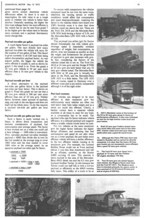
given above cannot determine vehicle efficiencies either. In short it is next to meaningless. Its only value is as a rough guide to whether one vehicle is better than another. Generally speaking, the higher the time-load-mileage factor the more efficient is the vehicle but as can be seen from graph 7 at the higher gvw the values tend to become more constant and a payload discrepancy could change that.

Payload ton-miles per gallon A much better factor is payload ton-miles per gallon. This says directly how many payload ton-miles the vehicle will carry for the expense of one gallon of fuel. This factoiis given currently in all CM road tests being called characteristic payload factor. As was argued earlier, the bigger the vehicle the more efficient it usually is, and as shown by graph 5 this trend is so. From the graph a 32 tons gcw vehicle is 50 per cent more efficient than a 16 tons gvw vehicle in this respect.

Payload ton-mile per hour A direct alternative to the payload ton-miles per gallon factor is the payload ton-miles per hour factor. This is shown on graph 6. From this graph we can see that a 28 tons gvw vehicle is 300 per cent more efficient than one of 10 tons gvw. Neither factor, however, takes account of payload, mpg and mph in the one figure and does not itself tell the whole story. To do this requires a payload ton-mile per gallon per hour factor.

Payload ton-mile per gallon per hour Such a factor is easily worked out, is linear, ie allows direct comparison, and includes consideration of payload, fuel consumption and average speed. The factor is best worked out on a what one could call a base mileage — 1000 miles is convenient. First, calculate payload ton-miles (multiply payload x 1000) then divide this in turn by the fuel needed at the average mpg to cover 1000 miles and the time needed to cover 1000 miles at the average speed. As an equation payload ton-miles /gal /hr factor.

=payload x 1000 1000 x 1000

mpg mph =payload x 1000 x mpg x rflph 1000 1000 —payload x mpg x mph 1000

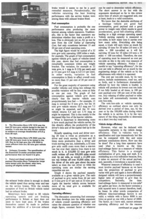
To ensure valid comparisons the vehicles compared must be run over the same route, otherwise the varying terrain or traffic conditions would affect fuel consumption and speed disproportionately. Applying the factor to the vehicles which were tested over CM's Scottish route it is clear that three vehicles stand out above the rest. These are the Ford DA 2418 and the Mercedes-Benz LPS 2024 both having a factor of 5.56, and the Mercedes-Benz LPS 1632 with a factor of 5.85.

The payload ton-miles /gal /hr factor should theoretically rise with vehicle gvw. Average speed is reasonably constant regardless of weight; fuel consumption, as shown, does not increase as quickly as does the weight and furthermore the proportion of payload to gvw also increases with gvw. In fact, considering the factors of the vehicles tested this is not so. The Ford DA 2418 at 24 tons gvw and the Dodge KT900 at 22 tons gvw are both better than any 32 tons gew vehicle tested. The Mercedes-Benz LPS 2024 at 38 tons gvw is virtually the same as the Ford, and the Mercedes-Benz LPS 1632 is a little better. The LPS 1632 was, of course, tested in Germany over a different route and is not strictly comparable although it is of the right order.

Part-load economy All vehicles are , designed to be most efficient at their maximum gvw but unfortunately most vehicles are often run well below their fully laden weight and as a result are much less efficient. Clearly, a haulier cannot have a separate vehicle available at all times to cater for any load, so a compromise has to be made. The payload miles /gal /hr factor indicates vehicle efficiency at a reduced payload and suggests when a smaller vehicle would better be used.

For two vehicles at the same maximum gvw the higher factor indicates the higher design efficiency and assuming that fuel consumption and speed do not alter when run at a lower payload, the part-laden more efficient vehicle will have a similar efficiency to the less efficient vehicle running at its maximum gvw. For example, the Leyland Redline Boxer could run at 9-ton payload (about 2 tons less than maximum) and still be as efficient, costwise, as the Scania LB80 carrying 10 tons. This exercise is more marked in the case of the MercedesBenz 406D diesel van and the 8.5 tons gvw Leyland Redline Terrier. In this instance the Terrier could run half full, ie with a 2.6-ton payload as efficiently as the 406D running fully laden. This ability of a truck to be as

Of the three vehicles tested at 38 tons gew the best was the Mercedes-Benz LP 1632 at 5.85 but is not strictly comparable as it was tested abroad. It seems that at or about 32 tons gm the proportion of unladen weight to gcw reaches a limit and is stationary thereafter if it does not actually decrease. The weight of larger engines, heavier chassis and extra axles bites into the extra payload bonus on these heavier vehicles.

If asked to nominate a top British-built truck from the vehicles tested in the last 12 months I would have to choose the Ford DA 2418. This truck has a very advanced specification and as a result has out-performed all the others. The DA 2418 has a direct-drive top gear and a single-reduction axle and again points to the importance of a high transmission efficiency. Not only does it perform well on paper for it is easy to drive and very comfortable; the noise level is the lowest of any heavy British truck tested. The best 32-tanner tested was the Mercedes-Benz LPS 1418 and the best British 32-tonner the ERF.

Group one and two have less vehicles in them but the Leyland Redline Terrier 850 is outstanding in its class and the Leyland Redline Boxer equally so in its class.

The foregoing will undoubtedly lead to some sharp correspondence but I feel the method of assessment is the most realistic applied to the vehicle selection problem so far. efficient at part load as others at full load is perhaps the most important single characteristic.

Of the nine 32-tanners tested it is significant that the best three are foreign. The best was the Mercedes-Benz LPS 1418 followed by the Volvo F86, then the DAF FT2600. Why did the British art ics perform worse than the foreign ones? The payload ton-miles /gal /hr factor is, as I have said', a measure of vehicle design efficiency and the simple fact is that British 32-tonners are heavy and dated in their design.

Much of the answer must, I feel sure, lie in transmission efficiency. All the British 32-tanners have overdrive top gears and double-reduction axles. Of the foreign 32-tanners the DAF FT2600 has an overdrive top gear and double-reduction axle and is, as an indication of the argument, only fractionally better than the ERF. The Volvo has a double-drive axle but a direct top. The Mercedes-Benz LPS 1418 has a direct-drive top gear and a two-speed axle. It would appear to follow that a high horse power lightweight 32-tonner having a direct-drive top gear and a single-reduction rear axle would, therefore, out-perform them all No such vehicle has been tested this year but last year CM did test a Scania LB80 Super at 32 tons gcw over the Scottish route and the factor for that vehicle works out to 5.75. That test was done before the 60-odd mile stretch of M6 between Carnforth and Carlisle was open and it is likely that figure could be improved upon now. A vehicle with a more powerful lightweight engine, say, the Mercedes-Benz V8 at 256 bhp or the Cummins 555 V8 at 240 bhp, together with the transmission described, would probably better a figure of 6.00