


Transport economics applying DCF
Page 61
If you've noticed an error in this article please click here to report it so we can fix it.
I EXPLAINED the theory of discounted cash flow (DCF) last week in view of its importance as a tool for transport management and the fact of its frequent occurrence in the more advanced transport economics examinations. The theory is relatively easy and much less terrifying than many seem to fear, but its application to specific road transport problems is rather more complex.
Suppose a vehicle manufacturing company invests a large sum of money in order to retool part of the plant so that it can produce a new specific type of van. The plant for this particular model is expected to remain for five years. The production is geared for sales of 1,000 vans a year selling at (to make the arithmetic simple) .€1,000 each. The value of the first year's vans will be £ lm. But the value in present-day terms of the second year's 1,000 vans is £1m less the rate of interest which could be earned on that £ lm in the time span between now and its arrival after one year. In the same way, the value now of the third year's £1m. is less the (accrued) rate of interest which could be earned on that £1m in the time span between now and its arrival after two years-and so on for five years.
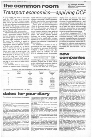
It is sometimes easier to look at these problems in statistical terms. Examining a slightly different example; suppose a fleet of vehicles costing Lim is used so intensively after five years that they have no further use, the problem can be tabulated as shown below.
Year 0 is the base year and the year in which the investment cannot produce any return. In this particular case there is only one capital expenditure, but, of course, in a normal transport situation, there would be capital outlays throughout the life of the project. Net returns represent operating surpluses but exclude depreciation and interest. Since the capital outlay is lumped together (in the second column) depreciation does not arise and interest is treated under the Discount factor.
The mathematics involved are not as mysterious as they might appear, in year 3, for example, the net return of £250,000 is multiplied by 0.794 to arrive at the Discounted return of £198,500. The factor 0.794 is calculated through the expression
(1 plus rate of discount)3 (1,08)3
remembering the rate of 8 per cent being the minimum accepted rate of return for the project and the sum is cubed since this is the third year being taken as the example.
The final total shows that as the figure is slightly below £1m, thus the target is less than the 8 per cent anticipated. The aim is, of course, to reach equilibrium on a particular project. Obviously many projects can be very complex arithmetically involving the use of many aids but the principles shown remain the same and can serve as a useful examination example to show the workings of the discounted cash flow technique.
In practical management, DCF is an invaluable tool for forecasting the timing and of receipts and costs. There is naturally a very close connection between this economic technique and orthodox financial budgeting. In transport examinations, students will not be expected to make the actual calculations but will be required to understand the use of discounted cash flow and how it can be applied.